
FPGA vs Microcontroller Silicon: Using Microarchitecture Transistor Counts to Distinguish Between LSI and VLSI Eras
Ever popped open a package, looked at a die photo under an optical microscope, and felt completely lost? You are not alone. Back in the day, figuring out what was happening inside an integrated circuit meant counting tiny physical gates or tracing aluminum interconnect lines by hand. Today, when comparing FPGA vs microcontroller silicon, the shear density of physical features makes your eyes bleed if you try to do it the old-fashioned way.
Here is the deal. Engineers love to throw around terms like LSI and VLSI as if they are static categories frozen in a 1980s textbook. But microarchitecture evolved at a breakneck speed, completely blurring those historical lines. If you look closely at microarchitecture transistor counts, you can actually draw a hard, mathematical boundary between the Large Scale Integration era and the Very Large Scale Integration age.
Look—it is not just about bragging rights for chip design teams. Understanding how logic density shifted over time tells us why modern microcontroller silicon evolved to look like a messy bento box, while an FPGA silicon layout looks like a hyper-repetitive crystal lattice. Let us tear down the silicon, count the raw gates, and make sense of this architectural leap.
Honestly? It is a fascinating trip down physical layout memory lane.
Deconstructing the Silicon Scale: From LSI Density to VLSI Complexity
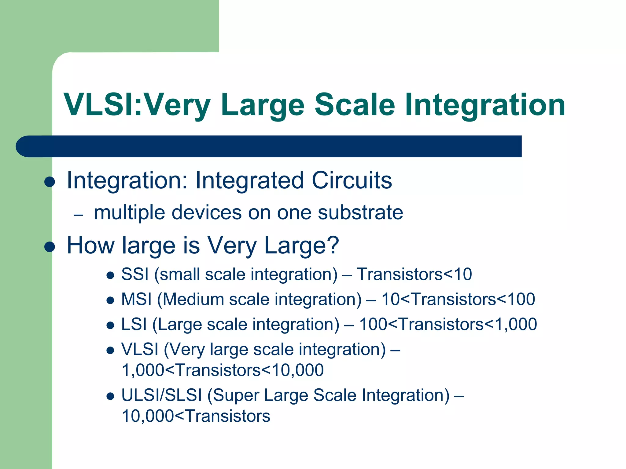
To understand where the shift happened, we have to look back at the actual transistor math on the substrate. The Large Scale Integration (LSI) era was defined by bringing thousands of discrete components onto a single piece of silicon. We are talking roughly about 1,000 to 10,000 transistors per chip. Think of classic 8-bit CPUs that powered early computing, where every single register and ALU bit-slice was manually drawn by a human draftsman on Mylar sheets.
Then, the floodgates opened. Very Large Scale Integration (VLSI) pushed transistor counts beyond the 100,000 mark, eventually soaring into millions and billions. This leap was not just a manufacturing victory; it fundamentally altered how silicon real estate was allocated. In an LSI microarchitecture, every single transistor had a explicit, dedicated job for a specific logic instruction. In VLSI, density became so cheap that designers started "wasting" millions of transistors on regular structures like SRAM caches, routing grids, and programmable lookup tables.
The distinction matters immensely when analyzing LSI and VLSI eras through a modern lens. In early chips, logic density was hard-wired and scarce, forcing hyper-optimized instruction sets. As process nodes shrunk past the 1-micron barrier, the raw gate count exploded, allowing designers to trade sheer area efficiency for architectural flexibility. This critical pivot point is precisely where the evolutionary paths of microcontrollers and FPGAs split forever.
So, how do you tell these eras apart just by looking at a die? It comes down to raw structural organization. LSI layouts display visible, custom-designed logic blocks with chaotic routing channels snaking between them. VLSI layouts, conversely, are dominated by rigid array structures—massive banks of identical memory cells or hyper-dense, repeating logic tiles separated by uniform copper bus networks.
Defining the Structural Metrics
- LSI Scale: Roughly 1,000 to 10,000 transistors featuring custom, hand-routed standard cells.
- VLSI Scale: 100,000 to tens of billions of transistors driven by automated synthesis and place-and-route tools.
- Functional Area Allocation: LSI chips dedicate up to 80% of silicon to active computing logic, whereas VLSI chips dedicate vast swathes to interconnect structures, arrays, and onboard memory.
- Defect Tolerance: High-density VLSI architectures require redundant silicon pathways, unlike their leaner LSI predecessors.
The Transistor Count Threshold
The line between these two eras is not arbitrary; it represents a fundamental change in chip synthesis. When a design crosses the ~100,000 transistor boundary, human-driven manual placement becomes physically impossible. Computer-Aided Design (CAD) software takes over. That transition alters the physical signature of the silicon itself.
You can spot a CAD-synthesized VLSI layout instantly. The random, organic flow of hand-drawn LSI logic gates gives way to highly stylized, rectangular blocks of automated logic. It is the exact moment when silicon engineering stopped being an artisanal craft and became a software-driven science.
Without this threshold, modern programmable logic simply could not exist. The sheer mathematical overhead of routing signals dynamically requires a transistor budget that absolute dwarf the basic logic functions being performed. LSI just did not have the physical real estate to make that trade-off work.
Microcontroller Architectures: Hard-Wired Efficiency in Silicon
Let us talk about modern microcontrollers. A typical microcontroller unit (MCU) represents the ultimate evolution of deterministic, domain-specific silicon. Whether you are looking at a classic 8051 or a modern ARM Cortex-M4, the underlying philosophy remains fixed: maximize efficiency by hard-wiring functional blocks directly into the substrate. There is almost zero wasted spatial capacity inside an MCU die.
In a standard microcontroller layout, the central processing unit occupies a surprisingly small fraction of the total surface area. The rest of the die is packed with onboard peripherals—Analogue-to-Digital Converters (ADCs), timers, UART channels, and non-volatile flash memory. Each of these modules is implemented using specialized standard cell libraries optimized for minimal transistor counts and ultra-low leakage current.
Because these blocks are fixed, the overall microarchitecture maintains an exceptionally tight functional density. An ALU bit requires a precise, minimal number of physical MOSFETs to compute an operation. You do not get the dynamic reconfigurability of an FPGA, but in return, you get extreme power efficiency, instantaneous boot times, and predictable deterministic performance. It is a dedicated instrument built for a single, unyielding purpose.
When measuring transistor density in FPGAs versus microcontrollers, the MCU wins hands down on logic per area for fixed tasks. Every transistor is optimized for its exact placement. A 32-bit adder in an MCU uses only the exact number of gates needed to execute that arithmetic instruction—not a single transistor more.
Core Components of MCU Silicon
- Integrated Hard IP: Dedicated silicon blocks for SPI, I2C, PWM, and analog comparators that operate independently of the main core.
- On-Chip Embedded Flash: Non-volatile memory banks integrated directly alongside control logic using high-voltage process extensions.
- Static RAM (SRAM): Dense, low-leakage 6-transistor (6T) cell arrays built for ultra-fast register access.
- Control and Bus Logic: Hard-wired multiplexers and bus matrix crossbars for deterministic data movement.
The Economic Logic of Fixed Silicon
Hard-wired logic is cheap to mass-produce. Once the lithography masks are finalized, printing ten million units of a fixed MCU die costs pennies per square millimeter. There is no programmable interconnect overhead cluttering up the substrate.
However, this rigidity is a double-edged sword. If you discover a bug in a hardware timer block, or if an industry protocol shifts, that silicon is permanently obsolete. You cannot push a firmware update to rewire physical silicon traces inside an MCU core.
This reality forces MCU designers to rely on proven, stable digital logic architectures. Consequently, microcontrollers often retain structural design cues from late-stage LSI and early VLSI designs, prioritizing raw reliability over experimental configurable layouts.
FPGA Silicon Layouts: The Overhead of Universal Reconfigurability
Now, flip the coin and look at an FPGA under a microscope. It looks completely alien compared to an MCU die. Instead of a heterogeneous collection of distinct peripheral blocks, an FPGA die is a vast, repeating ocean of identical Configurable Logic Blocks (CLBs) surrounded by a massive matrix of programmable routing channels. It is the absolute pinnacle of high-density VLSI engineering.
Here is the mind-blowing part: the actual logic in an FPGA—the Lookup Tables (LUTs) and Flip-Flops that do your actual work—occupies only a tiny fraction of the total transistor count. The overwhelming majority of transistors on an FPGA die are spent on the reconfigurable interconnect architecture. Pass transistors, transmission gates, and SRAM configuration cells dominate the layout just to allow a signal to travel from point A to point B.
Consider a simple 4-input NAND gate. In a microcontroller, you can build that using four tiny MOSFETs. In an FPGA, implementing that same NAND gate requires configuring a LUT, which relies on a multi-bit SRAM array, multiplexing tree logic, and multiple programmable routing switches. That single logic function might consume hundreds of active transistors behind the scenes! That is the price of total reprogrammability.
This massive multiplier effect explains why FPGAs jumped headfirst into advanced VLSI process nodes far earlier than microcontrollers. To make programmable logic commercially viable, manufacturers had to wait until deep-submicron manufacturing provided millions of cheap, low-power transistors to burn on routing overhead. Without true VLSI density, an FPGA is simply too inefficient to exist.
Structural Breakdown of an FPGA Die
- Configurable Logic Blocks (CLBs): The basic building blocks containing SRAM-based LUTs, full adders, and dedicated flip-flops.
- Programmable Routing Matrix: Horizontal and vertical wiring tracks interconnected by programmable switch boxes (S-boxes) and connection boxes (C-boxes).
- Specialized Block RAM (BRAM): High-density dual-port memory matrices dispersed throughout the logic array for high-bandwidth local storage.
- Digital Signal Processing (DSP) Slices: Hardened silicon multiplier-accumulator units integrated directly to accelerate complex math functions.
The Spatial Penalty of Reconfigurability
That insane interconnect infrastructure comes with a steep physical cost. Signals traveling through programmable switch matrices encounter significant parasitic resistance and capacitance. This physical reality makes FPGAs inherently slower and far more power-hungry than an equivalent hard-wired ASIC or microcontroller executing the exact same gate logic.
Seriously, the parasitic losses alone are staggering. You are essentially forcing signals to cross dozens of microscopic pass-transistors just to move between adjacent logic gates. It is an operational nightmare from a pure physics standpoint.
Yet, the ability to completely mutate your hardware microarchitecture in a few milliseconds makes that spatial penalty worthwhile. You are trading raw physical layout efficiency for absolute functional agility—a classic VLSI-era compromise.
Transistor Count Comparison: Hard-Wired Logic vs. Programmable Gates
Architectural Parameter Standard Microcontroller (MCU) Field Programmable Gate Array (FPGA) Dominant Integration Era Late LSI to Early VLSI Paradigms Ultra-Dense Modern VLSI Era Transistor-to-Logic Ratio Near 1:1 (Direct functional implementation) Up to 100:1 (Interconnect & LUT overhead) Silicon Allocation Strategy Heterogeneous dedicated peripheral blocks Homogeneous repeating logic and routing matrix Substrate Utilization Extremely high logic density per mm² Low effective logic density; dominated by routing Power Dissipation Profile Ultra-low static and dynamic leakage High baseline power due to switch capacitance
Determining Historical Eras Through Gate-Level Diagnostics
So, how do we use these silicon traits to reverse-engineer where a target chip sits on the LSI-to-VLSI spectrum? It starts with analyzing physical die parameters using high-resolution electron microscopy or optical delayering techniques. By quantifying gate density, interconnect metal layers, and structural symmetry, you can map the design straight to its historical microarchitecture class.
First, take a look at the metal stack. Early LSI designs were severely constrained by single-layer or double-layer metal interconnects (typically aluminum). This forced designers to route signals directly through the active silicon layer using polysilicon runners, which added huge resistance. If your die photo shows wide, manual routing paths constrained to just two metal levels, you are staring right at an LSI-era architecture.
Modern VLSI chips—especially FPGAs—look like hyper-dense skyscrapers in cross-section. They utilize 10 to 15+ layers of copper interconnects. The top layers handle low-resistance power distribution, while the dense lower metal layers construct the complex routing networks. The presence of dense, multi-tiered interconnect fabrics is a definitive marker of mature VLSI scaling.
Second, measure the ratio of raw logic area to memory/routing area. In an LSI microarchitecture, memory is a rare luxury. Early microcontrollers used primitive flip-flop arrays or minimal register files. If the silicon surface is dominated by complex, asymmetric control logic with minimal uniform arrays, it fits squarely into the LSI paradigm. If it is dominated by massive repeating grids, you are safely in VLSI territory.
Finally, inspect the symmetry of the logic array. An FPGA presents extreme spatial auto-correlation—a mathematical way of saying that one square millimeter of the die looks identical to the next. Microcontrollers present localized symmetry inside specific blocks (like SRAM or Flash), but maintain a highly chaotic overall global layout. This metric allows automated computer vision tools to instantly classify die photos without needing proprietary schematic files.
Diagnostic Signatures of Chip Eras
- Single/Dual Metal Layers: Unmistakable signature of original LSI era manufacturing.
- Chaotic Standard Cell Routing: Signals hand-drawn or laid out via early auto-routers indicate transitional LSI/VLSI designs.
- High Spatial Auto-Correlation: Highly uniform grids indicate an FPGA built on deep-submicron VLSI processes.
- Integrated Hard MAC Slices: Indicates modern heterogeneous VLSI system-on-chip (SoC) architectures.
The Future Boundary
As we push past traditional silicon lithography into 3D stacked dies and chiplet architectures, the historical definitions of LSI and VLSI are evolving again. Advanced packaging techniques let engineers stack an FPGA logic fabric directly on top of an MCU bus matrix using micro-bumps.
When distinct silicon architectures merge in three-dimensional space, the old transistor-counting rules get complicated. Yet, the core physical truth remains immutable.
Whether you trace logic through a single layer of aluminum or a 12-layer copper stack, the raw geometry of the silicon never lies. The spatial overhead of reprogrammability will always separate true field-programmable logic from hard-wired microcontrollers.
Common Questions About FPGA vs Microcontroller Silicon
What is the primary physical difference between FPGA and microcontroller silicon?
The main physical difference lies in their internal silicon layout. Microcontrollers use hard-wired, dedicated standard cell logic optimized for specific functions, resulting in high functional density and low spatial waste. FPGAs consist of a repeating grid of programmable Lookup Tables (LUTs) and logic blocks dominated by a massive, reconfigurable SRAM-based routing matrix.
Why do FPGAs require higher transistor counts than microcontrollers for the same operation?
FPGAs require significantly more transistors because of the architectural overhead of universal reprogrammability. Implementing a single simple logic gate in an FPGA requires configuring underlying SRAM configuration cells, multiplexers, and multiple pass-transistors within the routing array, whereas a microcontroller implements that same gate with just a few dedicated, physical MOSFETs.
How does transistor count define the transition from LSI to VLSI eras?
The transition from Large Scale Integration (LSI) to Very Large Scale Integration (VLSI) occurs around the 100,000-transistor mark. Beyond this threshold, manual human layout becomes physically impossible, forcing the industry to adopt computer-aided design (CAD) tools, automated synthesis, and regular, array-based silicon structures such as memory grids and programmable interconnect fabrics.
Can you classify a chip era just by examining a die photo?
Yes. You can classify chip eras by inspecting parameters such as metal interconnect layers, layout symmetry, and array repetition. LSI chips exhibit visible, asymmetrical, hand-routed logic channels with minimal metal layers. VLSI chips, particularly FPGAs, are characterized by ultra-dense multi-layer copper interconnect stacks and highly symmetric, repeating logic or memory arrays.